12.7. Sequential Adjustments with Tracking ID

This section of the manual steps the user through each sequential network adjustment required for submission to NGS.

12.7.1. Preliminary Adjustment

Recall that the Preliminary Adjustment is a minimally constrained geometric (3D) adjustment that combines the baseline vectors from the session solutions into one network and creates the files needed as input for the subsequent adjustments. This is a good opportunity to gauge how well the overall network adjustments will be, as the solutions should not change very much in the subsequent steps. In other words, this is a good opportunity to quality assure the overall project.

12.7.1.1. Setting up the Preliminary Adjustment

In the Network Adjustment window, select the available solutions from session processing that you want to include in the adjustment. Do not include more than one solution for a given session (see explanation of Session vs Solution in Section 11.3 and in the Glossary).

Caution

Although all sessions are typically included in the Preliminary Adjustment (and subsequent adjustments), this is not always the case. In rare instances, one or more sessions may be excluded due to poor fit, or unresolved errors in the corresponding observations.

OP will offer what it believes to be the best constraint: usually a CORS, used as a hub during session processing, close to the center of the project which it believes will provide the best solution. The user can easily change the constraint. If another CORS or mark is preferred, make sure to return the originally selected CORS to CONSTRAINT = NONE. Select only one mark/CORS in this preliminary adjustment, even if you have more than one hub, this is illustrated in Fig. 12.15.

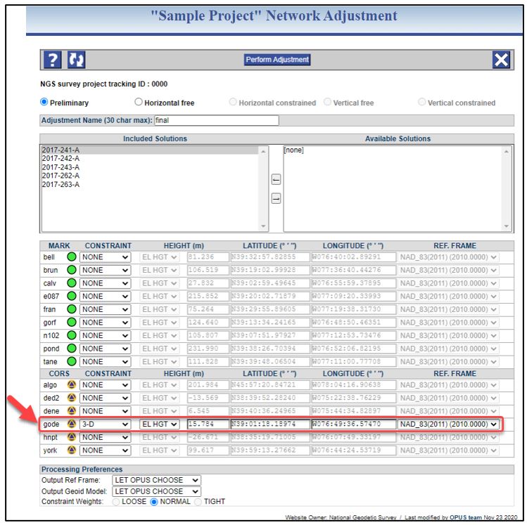
Fig. 12.15 Preliminary Network Adjustment window showing OP recommendation for a single hub 3D constraint

Caution

REF FRAME should be the latest realization of the NSRS if submitting to NGS for publication.

12.7.1.2. Analyzing the Preliminary Adjustment

Review the Processing Report (*.txt). Check to make sure the standard error of unit weight is near 1.0. Verify the total number of marks and that only one mark was constrained horizontally.

The MARK ESTIMATED - A PRIORI COORDINATE SHIFTS represent the shifts from the original a priori coordinate to the new session-adjusted coordinate. The a priori coordinates either come from published datasheets (CORSs and user marks with published coordinates) or from the first OPUS solution seen by the project (user marks that do not have published datasheets). Shifts should be small (smaller than ±2 cm horizontal and ±4 cm vertical). If poor results are indicated (a priori shifts are large), go back to session processing to see if you can find the offending observation (and exclude it). Refer to Solution Statistics (Section 11.5) to compare among sessions. Also consider collecting the .vec results into a single text file or spreadsheet and compare among repeat vectors for consistency. See Appendix C, Coordinate Shifts, for more details on shifts and their interpretation. Be careful to ensure at least two occupations remain. If everything looks good, move to the horizontal free adjustment.

Caution

If all the (a priori) coordinate shifts are similar in magnitude and direction, it is possible that the constraint is biased. Verify the position of the CORS used as the hub. You may try rerunning the adjustment with a different constraint.

12.7.2. Horizontal Free Adjustment

This step aligns the project to the NSRS reference frame. The overall goal is to verify that the field observations and satellite data have produced a set of baseline vectors that agree with each other and which can be aligned to published control in a horizontal constrained adjustment.

12.7.2.1. Setting up the Horizontal Free Adjustment

From the Network Adjustment window, select the Preliminary Network Solution and any GVX files in your project, as shown in Fig. 12.16. Then use the arrow key to transfer them to the left window. OP will suggest the same constraint that was used in the Preliminary Adjustment (hub station in 3-D). If any changes were made to the suggested constraint, it should be mirrored here as well.

When adding GVX files to your Horizontal free adjustment, you may receive a message informing you that your project has “disconnected subnetworks’’. This is because the data truly are disconnected into smaller networks. The software will recommend one constraint for each subnetwork, to provide minimal control to each of the subnetworks. You may wish to select other stations as constraints (by changing the constraints dropdown list), but a minimum of one constraint is needed for each subnetwork or the adjustment cannot run.

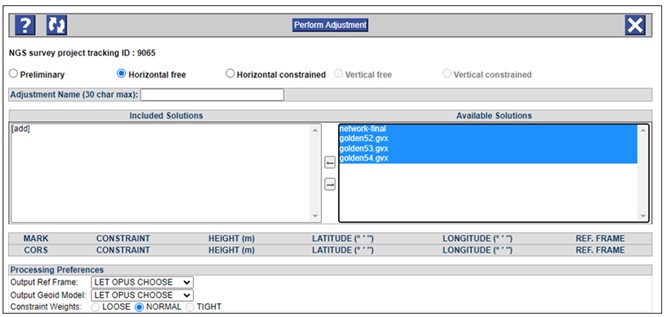
Fig. 12.16 Setting up the Horizontal free adjustment with both the Preliminary adjustment results and GVX files.

12.7.2.2. Analyzing the Horizontal Free Adjustment

Review the summary file provided in the body of the email, which is also given in the Processing Report (.txt), and the Processing long (.sum) . Verify that the standard error of unit weight is approximately equal to 1.0. Check the total number of marks and make sure that only one mark was constrained horizontally. Review the MARK ESTIMATED - A PRIORI COORDINATE SHIFTS table. In this instance, the shifts are from the Preliminary to the Horizontal Free adjustments. A well fitting Horizontal Free adjustment will result in small coordinate shifts and low residuals on all observations, ideally ≤ 2 cm horizontal and ≤ 4 cm vertical for both. If this is not the case, then the user should review the Processing Log (below).

Processing Log (.sum):

Review the 20 greatest residuals: residuals exceeding ±2 cm horizontal and ±4 cm vertical indicate poorly fitting observations or a poorly fitting mark. For stations with more than two occupations, it is usually obvious which is the outlier. If an outlier is found, try to resolve the issue by checking field logs, setup photos, or conferring with the observer to rule out blunders in the field procedures. If there is no obvious cause, you will have to decide whether to remove the observation(s) or mark(s) from the project, or live with a large residual. Care should be taken to prevent a user mark from becoming no check as explained earlier. It may be a good idea to obtain an additional observation on the mark in question. If this is not possible, it may be necessary to remove the user mark from the project.

COMPVECS Output:

Look for large differences among replicate vectors.

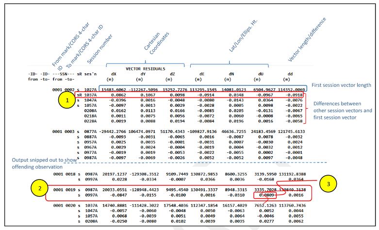
Fig. 12.17 Sample COMPVECS output showing: (1) a rejected vector; (2) a session (0987A) with large residuals; and (3) the large residual in the “Up” direction

The first two columns indicate the vector “from” and “to” marks as described by the four-character IDs assigned to the marks and CORSs in the project. The third and fourth columns identify the marks and CORSs by their Station Serial Numbers (SSNs). The fifth column indicates whether the direction of the vector is reversed. The sixth column gives the session number (three-digit GPS day followed by the last digit of the calendar year, followed by the session ID for that day).

Although the COMPVECS file itself is not easily sorted, it can be searched for particular values (e.g. 0.05). If one session appears to result in consistently large differences, take a closer look at that session to see if you can pinpoint an offending observation. If no errors can be found, you may have to remove that occupation from the analysis and re-process (remember - for submission to NGS, you will need at least two observations per mark).

Fig. 12.17 shown above gives an example of a rejected vector: the letter “R” to the right of the s/R column for vector SSN 0001-0002, session 1037A (#1 in the figure above). Note that the residuals for this vector are uniformly large.

The example also shows where the large residual in the “Up” coordinate in Session 0987A came from (seen previously in the *.sum output in Section 12.7.2): vector 0001-0019, session 0987A (#2 and 3, above).

At this point, if you have isolated an offending observation, or an offending user mark, you will have to decide whether to reprocess, remove the observation or user mark from the project, or accept the large residual. In the example shown in the COMPVECS table, there are only two observations for the user mark 0019 (“TUET”), so it would be only a guess at which is the bad one. Furthermore, there must be multiple occupations on each user mark so removing one is not an option in this example. Try to resolve the issue. Double check field logs to ensure no blunder exists.

For stations with more than two occupations, it is usually obvious which is the outlier. Inspect the computed minus observed (C-O) residuals in the ADJUST output (see Processing Log or *.sum file). List any outliers in the project report. Attempt to reduce large residuals (e.g. exceeding 2 cm horizontal and 4 cm vertical) by resolving any errors or removing offending observations. Note that these values are guidelines, not rules: refer to your project specifications for specific tolerances.

Below the table of comparisons is a histogram plotting the unadjusted vector differences from the COMPVECS output. The distribution should approximate a bell-shaped curve. Large outliers should be visible, and help the user identify the corresponding residual(s) back in the Processing Log. An example given below (Fig. 12.18) is for a histogram in the East component.

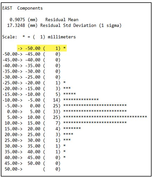
Fig. 12.18 Example of a histogram plotting the unadjusted vector differences from the COMPVECS output

If any observations are changed or removed, the corresponding session will be nullified and must therefore be reprocessed. Rerun the preliminary adjustment, and then the horizontal free adjustment. Repeat this process as necessary until you are satisfied with the results of the free adjustment.

PrePlt2:

PrePlt can be used to import residuals into a spreadsheet for sorting and identification of observations with large (positive or negative) residuals (see Section 12.7.4).

Final thoughts on the Horizontal Free Adjustment

After the completion of the horizontal free adjustment analysis, if large residuals remain, they should be listed in the project report, if the project is submitted to NGS. Likewise, all research on the cause of the residuals should be noted/explained in the report.

If any observations are changed or removed, the corresponding session will be nullified and must be reprocessed. If you wish to submit the project to NGS, you will need to rerun the preliminary adjustment, and then the horizontal free adjustment. Repeat this process as necessary until you are satisfied with the results of the free adjustment.

Finally, this is a good time to review the CHKOBS and OBSCHK output (12.7.5 and 12.7.6). If there are any errors at this stage, they will most likely not go away after any subsequent adjustments. Take the time now to see if they can be resolved. Contact the NGS Bluebook team, if needed, for help in resolving any errors.

12.7.3. Horizontal Constrained Adjustment

The function of this adjustment is to align the observed network with the previously-determined (published) coordinates of passive marks and CORS. The analysis focuses on absolute and relative measures of such an alignment. The results tell you how well your project fits within the existing NSRS.

12.7.3.1. Setting up the Horizontal Constrained Adjustment

On the Network Adjustment page (Fig. 12.19), select the Horizontal Free solution from the “Available Solutions,” and bring it to the “Included Solutions.” OP will offer all CORSs and user marks with published, geometrically (“3D”) adjusted coordinates as constraints in this adjustment step.

Caution

All constraints used in the Horizontal Constrained Adjustment must be held fixed in 3D.

Fig. 12.19 Sample Horizontal Constrained Adjustment window showing 3-D constraints

Change the distant CORS to “NONE” (recall that this CORS is for tropospheric modeling). As before, verify all elements of the window prior to processing. Perform the adjustment.

12.7.3.2. Analyzing the Horizontal Constrained Adjustment

There are several, if not many, factors to consider in the analysis of a constrained adjustment. The same output files and tools available in the free adjustment are produced in this adjustment with the exception of COMPVECS, OBSCHK, and CHKOBS checking programs. Although we still analyze vector residuals, we focus on the effects that the constraints have had within the network.

Tip

Finding an optimum alignment between an observed network and published control is an iterative process and users may find more than one satisfactory solution

F-test

In the main body of the email (Processing Report), the user will note the presence of an F-test (“F STATISTIC TEST” shown in Fig. 12.20).

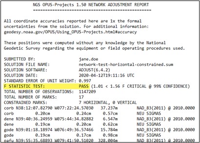
Fig. 12.20 Processing Report from the Horizontal Constrained Adjustment showing the results of the F-Test

Once the adjustment has been deemed acceptable i.e. all shifts and residuals are reasonable, the F-test should pass. The F-test is a statistical test which helps determine if the variance (variance of unit weight) from a fully constrained adjustment is significantly different from the variance (variance of unit weight) of a minimally constrained adjustment. The variance of unit weight is a critical statistic and should be looked at carefully when evaluating adjustment results. If the fully constrained adjustment fits well with all selected control (the constraints), the value of the variance of unit weight should be close to 1.0. The F-test is performed using a 99% confidence level.

If the F-test fails, it is due either to the errors (sigmas) of the constraints being overly optimistic (too small) or the constrained coordinates not agreeing with the observations (causing excessively large shifts of the constrained coordinates). Failure of the F-test does not automatically mean the constrained adjustment is bad. It is a flag that indicates there may be a problem with the constraints, and that they should be investigated. In addition, the F-test is based on the assumption of a normal (“bell-shaped”) probability distribution of the residuals. Networks with a distribution that is significantly non-normal may fail for that reason, even when a constrained adjustment is acceptable.

Since the F-test only gives information about the entire network, if it fails, it is necessary to inspect the network for specific stations that may be causing the failure. A convenient way to do that is provided in the next item (see Constraint Ratio). It may also be necessary to review the horizontal-free adjustment for possible causes.

Constraint Ratio

If the F-test fails, it is possible that some constraints need to be freed up. It might be the case where some of the shifts are too large. The Constraint Ratio (CR) test provides a way of identifying where the bad shift might be. The CR is essentially a Students T Test, with the absolute value of the shift between the adjusted, constrained coordinates and the published coordinates, divided by the sigma (σ, or standard deviation) used to constrain the station. It is computed for each component (north, east, and height):

\(|Adjusted coordinate - published cooridnate|/\sigma\)

OP provides the CR for all marks in the final table in the output summary given in the body of the email or in the Processing Report (.txt), as shown below in Fig. 12.21.

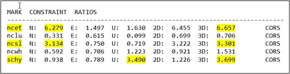
Fig. 12.21 Constraint Ratio Test as seen in the Processing Report of the Horizontal Constrained Adjustment

The computed CRs are compared to the critical value or 3.0, corresponding to a T-statistic at a 99% confidence level. If the value of CR is greater than 3.0 for any of the three components, that indicates that there may be a problem with the constrained station.

If a constraint is deemed problematic, then all three components (lat, lon, ellipsoid height) should be unconstrained in a new Horizontal Constrained adjustment. However, failure of the F-test or CR > 3 does not necessarily require removal of constraints. Both tests are analysis tools that only indicate potential problems; they are not substitutes for professional judgment. However, the reason for either failure occurring in the final constrained adjustment should be explained in the report.

Caution

A high constraint ratio could be simply due to a very low sigma

Unrealistically small sigma values could result in a warping of the network to fit constrained marks. For this reason, it may be better to free up (release) constraints with CR > 3 for any of the three components. It may be a good idea to review the values for sigmas under Section 7.3.12 “Manage Coordinates,” but it is not advised to change them unless they are known to be inaccurate. Freeing an offending constraint is typically the best strategy.

Note your findings in the project report. It may be that a station needs to be freed for the sake of the adjustment, but the newly computed position may not necessarily be updated in the NGS database.

If any constraints are freed, the F-test results should improve. However, users should review the newly adjusted coordinates on user marks to decide if they recommend the user mark be re-determined (re-published). Typically, this would happen if the coordinates have shifted by more than 2 centimeters horizontally or 4 cm vertically from the published coordinates.

Coordinate Shifts

Best reviewed in the Processing Report (*.txt) or in the body of the email, there are two tables of shifts given. The first one represents the difference between where the Horizontal Constrained adjustment versus the Horizontal Free adjustment want the station to be (“MARK ESTIMATED - HORIZONTAL FREE ADJUSTMENT COORDINATE SHIFTS”), as shown in Fig. 12.22.

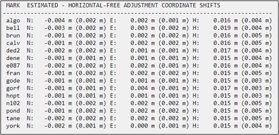
Fig. 12.22 Network solution processing report from the Horizontal Constrained Adjustment showing “MARK ESTIMATED - HORIZONTAL-FREE ADJUSTMENT COORDINATE SHIFTS”

Large shifts (> 2 cm horizontal and > 4 cm vertical) are an indicator that one or more constraints may not fit the current network. Note that all marks in the project are listed in the table.

The second table represents the shifts between the Horizontal Constrained Adjustment and the marks with published (3D) coordinates (“MARK ESTIMATED - PUBLISHED HORIZONTAL COORDINATE SHIFTS”), as shown in Fig. 12.23. Note that only the marks which were constrained 3D are given in the table (these were the marks with adjusted/published 3D coordinates).

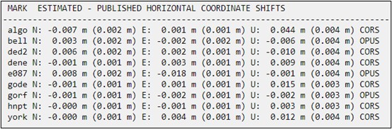
Fig. 12.23 Network solution processing report from the Horizontal Constrained Adjustment showing “MARK ESTIMATED - PUBLISHED HORIZONTAL COORDINATE SHIFTS”

If there are a couple large shifts compared to published coordinates (> 2 cm horizontal and > 4 cm vertical), that may suggest that the published coordinates may no longer match the marks positions. Many large shifts may be indicative of a bias in the hub (which should be very rare): this would require re-processing the sessions with another hub selected.

Residuals

The residuals (computed - observed or C-O values) are found in the main body of the Processing Log (.sum), see Fig. 12.24 for an example. Residuals are summed up in the min/max V values and 20 greatest residuals as described earlier in the Horizontal Free output (also see Section 12.7.2). Often you can see that the largest residuals will also appear problematic in the COMPARISON OF ADJUSTED AND CONSTRAINED COORDINATES AND HEIGHTS table which shows shifts between the constrained and the adjusted values of a mark. Large shifts in this table should be analyzed and addressed in the project report.

Fig. 12.24 Computed - Observed residual values shown in the processing log output for the Horizontal Constrained Adjustment

Other important results to verify:

Review the network accuracies in the Processing Log (*.sum file) for any indication that some user marks or CORSs might be problematic. Although network accuracies should be less than 2-4 cm, high variability among the accuracies may be more of a problem. Consistently large numbers (e.g. greater than 2 cm) would be less problematic than some values less than 1 cm and others greater than 4 cm. Note that horizontal network accuracies should always be less than vertical accuracies, and that network accuracies for CORSs are usually less than for user marks. An example of the reported network accuracies are shown in Fig. 12.25.

If the adjustment is still unable to produce a passing F-test, the user may find it helpful to re-run the Horizontal Constrained adjustment constraining only CORS as constraints (except for the distant CORS). This helps isolate possible problems with the passive control (user marks). The user would then compare the resulting position differences between the fully constrained and the CORS-only constrained adjustments. Looking at the user mark shifts between the two adjustments can help identify published user marks that no longer fit the NSRS.

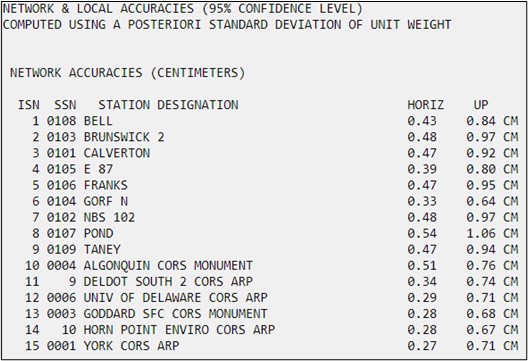
Fig. 12.25 Network accuracies as shown in the Processing Log

Unconstraining and re-adjusting

To re-determine a user mark, the user will have to re-run the Horizontal Constrained adjustment. Accessing the Network Adjustment window, OP will be expecting the next adjustment in the sequence (“Vertical free”). However, the user can re-select “Horizontal Constrained,” and proceed.

When you are satisfied with the constrained adjustment results, proceed to the next step to run the Vertical Free adjustment.

Caution

If the default Project Tracking ID “0000” is used and alignment to a vertical datum (e.g. NAVD 88 in the continental USA) is not required, or marks with published heights in a separate vertical datum were not observed, the analysis is complete (no project submission to NGS).

Caution

If you want to submit your project to NGS for publication, all five (5) adjustment steps need to be run, regardless of whether or not you have observed marks with published vertical control

12.7.4. Vertical Free Adjustment

The vertical free adjustment is similar in philosophy to the horizontal free adjustment as it is now aligning the adjustment to the vertical datum.

12.7.4.1. Setting up the Vertical Free Adjustment

In the Network Adjustment window, “Vertical Free” should be identified, and the user should select the Horizontal Constrained solution and bring it to “Included solutions”, an example is shown in Fig. 12.26.

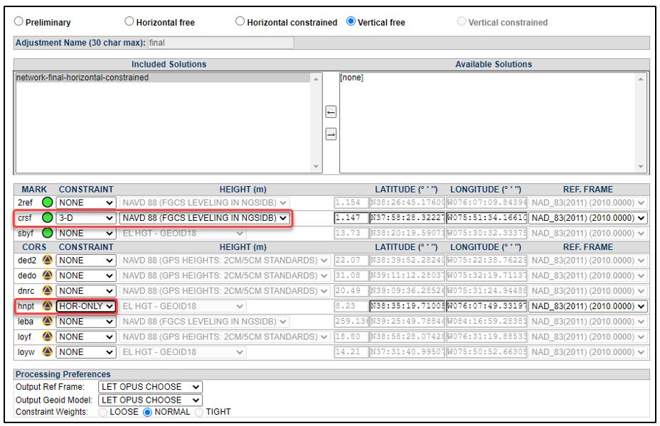
Fig. 12.26 Sample Vertical Free Adjustment constraint selection

OPUS will typically constrain horizontally the same mark that was used in the Horizontal Free adjustment (constraint now reads “HOR-ONLY”). It will also select what it believes to be the best orthometric height to constrain (“VER-ONLY,” typically a user mark with a high accuracy orthometric height published in the vertical datum, located centrally to the project). Note that there may be more than one “best” height to constrain, and the user may override the selection made by OP. Whichever constraint is used, make sure the height is correct.

Tip

If there are no published orthometric heights in the project area, OP will offer an orthometric height computed from the ellipsoid height and the geoid height: OH = EH - GH. However, these heights will not be published except in pre-authorized areas.

12.7.4.2. Analyzing the Vertical Free Adjustment

The results of the Vertical Free Adjustment are similar to that of the Horizontal Free adjustment. The summary information in the body of the email or the Processing Report (.txt file) are the best places to verify:

• Make sure there is only one horizontal constraint, and that the vertical constraint is the one that was intended.

• Ensure that the Standard Error of Unit Weight is 1.0.

• Ensure the coordinate shifts are small (VF vs. HC; there should be no surprises at this stage, if the prior adjustments fit well).

For completeness, the user may want to examine the differences between adjusted orthometric heights and published orthometric heights for all user marks which will be constrained in the next step (Vertical Constrained adjustment). Any large differences (e.g. > 4 cm) should be scrutinized prior to the VC adjustment. If there is any perceived systematic (vertical) bias, the user may want to select a different vertical constraint and re-run the vertical free adjustment.

If the results look good, the user will move to the final adjustment, the Vertical Constrained Adjustment.

12.7.5. Vertical Constrained Adjustment

As with the horizontal constrained adjustment the project is now being aligned with the local vertical datum. Heights used as control (constrained heights) will greatly affect the heights being determined. It is important that control has no adverse effects on the adjustment.

12.7.5.1. Setting up the Vertical Constrained Adjustment

In a similar manner as before, select the Vertical Free solution from the “Available Solutions.” OP will suggest the appropriate 2D (“HOR-ONLY”) constraint (or 3D, if the station has a published orthometric height), typically the same CORS or user mark used for horizontal control in the Vertical Free adjustment. OP will also suggest for constraint all user marks in the project that have appropriate published orthometric heights. An example is shown in Fig. 12.27.

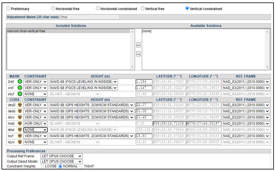
Fig. 12.27 Sample Vertical Constrained Adjustment constraint selection

Depending on the types of heights available in your area, there may be a number of possible types of vertical constraints in OP. The possible constraints are listed below.

Note that the blank space “_____” in the options below represents an official vertical datum published for the given mark/CORS. Examples include NAVD 88, PRVD02, GUVD02, etc. (see the NGS Vertical Datums table)

OP Vertical Constraint Options:

1. ______ (FGCS LEVELING IN NGSIDB): These are leveled heights that have been adjusted by NGS and are included in the datum network.

2. ______ (GPS HEIGHTS: 2CM/5CM STANDARDS): These are GPS derived heights that meet height modernization standards according to NGS 59 (see Glossary for more information).

3. ______ (FGCS LEVELING POSTED): These are orthometric heights established using FGCS leveling specifications and procedures, adjusted height is POSTED (pre-1991 precise leveling forced to fit the NAVD 88 data; excluded for various reasons from the NAVD 88 general adjustment).

4. ______ (LEVELING RESET): OP uses this term to describe two similar height sources:

1. LEVELING RESET: heights determined by differential leveling for classical horizontal observation reduction; reset procedures were used to establish the elevation, or

2. RESET: Third Order reset heights following reset specifications and procedures.

5. ______ (GPS HEIGHTS: DECIMETER ACCURACY): These are GPS derived heights that do not meet height modernization standards according to NGS 59 (see Glossary for more information). Use with caution.

Any of these five options (above) will meet the requirements of vertical constraints for submission to NGS. Two additional options exist, which are always available to the user when running vertical free and vertical constrained adjustments in OP (but never offered as a constraint by default). They should be used with caution. If submitting the project to NGS, their selection needs to be explained in the project report. Prior approval by NGS is recommended.

6. LEVELING NOT PUBLISHED: These are leveled orthometric heights that have been submitted to NGS which have not yet been loaded into the NGS database (aka “field heights”). This option is only available with prior approval.

7. EL HGT - GEOID__: Where GEOID__ is the current NGS geoid model published in your area. This may be the only option where orthometric heights are not available. Choose all stations used as control in the horizontal adjustment. OP will use the published Ellipsoid Height and subtract the geoid. The resulting heights will be published to the nearest cm. This option is not to be used as control in height modernization projects 4 .Use with caution. Note, these heights will not be published except in pre-authorized areas.

Once you have verified that all the constraints are correct, run the adjustment.

12.7.5.2. Analyzing the Vertical Constrained Adjustment

The analysis of the Vertical Constrained adjustment is similar to the one conducted after the Horizontal Constrained adjustment.

Tip

Finding an optimum alignment between an observed network and published control is an iterative process and users may find more than one satisfactory solution.

F-Test

In the main body of the email or near the top of the Processing Report (*.txt file), verify that the adjustment has passed F-test (“F STATISTIC TEST”). The F-test is a tool which allows you to detect possible issues with the heights you chose as constraints in the vertical constrained adjustment. If the F-test fails, there is additional output to scrutinize.

Coordinate Shifts

as shown in Fig. 12.28, there are three sources of heights to consider in this final step in the adjustments:

1. Adjusted orthometric heights that were constrained in the final adjustment

2. Adjusted orthometric heights from the vertical free adjustment

3. Published orthometric heights

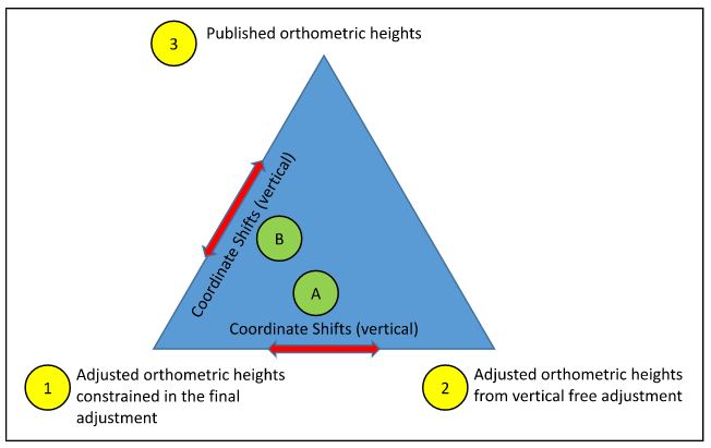
Fig. 12.28 Conceptual diagram showing relationship between adjusted heights from three different sources within OPUS Projects: the Horizontal Free Adjustment, the Horizontal Constrained Adjustment, and the published orthometric heights

In the interpretation of the results, keep in mind the estimated vertical sigmas that OP may have assigned to the vertical constraints. A larger vertical sigma may allow for larger shifts; see Appendix D for more information.

The first set of vertical coordinates to compare is between the VC and VF adjustments (A above). The coordinate shifts will be presented in the first table under “MARK ESTIMATED - VERTICAL FREE ADJUSTMENT COORDINATE SHIFTS.” Large shifts are indicative of poorly fitting vertical control.

If the vertical shifts are small, the next step is to compare the vertical coordinate shifts between the vertically constrained/adjusted heights and the published heights (B above). This is presented in the second table under “MARK ESTIMATED - PUBLISHED VERTICAL COORDINATE SHIFTS.” Large shifts may indicate poor control that may have to be freed up for the best-fitting adjustment.

Once the adjustment output looks good, confirm it has passed the F-test to ensure that the vertical constrained adjustment fits well with the identified vertical control. The Standard Error of Unit Weight should be close to 1.0. Review the constraint ratio analysis if the F-test fails.

Residuals

The residuals (computed - observed or C-O values) are summed up in the min/max V table found near the end of the Processing Log (.sum) as described earlier, along with the 20 greatest residuals. The DU values are representative of the vertical adjustment.

Caution

Note that some large residuals may be due to differences in the geoid models used to determine heights. If enough control exists it may be worth taking the opportunity to update the height on a mark

If all the results look good, you are ready to submit your project to NGS!

Tip

If the user wishes to download/copy the results of the final adjustment, they should be found in an output called “[adjustment name]-FINAL.” which is only available under the “Show File” button on the Manager’s Page (it is not included in any email attachments)

12.7.6. Final Steps

Prior to submission of the project to NGS, two final steps remain: uploading the final project report, and running the final checks.

12.7.6.1. Final Project Report

Upon completion of the adjustments, the project report should be finalized. A good report builds on the original proposal, providing the purpose and rationale for the survey. The report needs to identify who the work was performed for ( if other than the submitting agency), who performed the field work as well as the processing and adjustments. Most importantly, the report provides details of the analyses, including the identification of any published coordinates that were freed up in the adjustment, and providing explanations for any preferences that were not met. Below is a listing of the major elements to be included in the final project report:

• Cover Page:

  • Project name and tracking ID

  • Geographic location

  • Reference Frame/Datums to which the project was aligned

  • Submitting agency name and 6-char agency ID

  • If applicable:

    • On whose behalf the survey was performed for

    • Agency that performed the observations

    • Agency that performed the adjustment

  • Point of contact (name, physical address, telephone number, email address)

  • Date of report

  • Version of OPUS Projects

• Report:

  • The purpose of the survey and if any other agencies are involved and their roles.

  • A brief chronology of field work including reconnaissance, mark-setting, and observations

  • Procedures (timing of planned sessions and duration)

  • Sketch

  • Project Specifications

  • Table of user marks: both those marks used as control in the project w/ PIDs and new marks w/o PIDs

  • Table of equipment used (model numbers and serial numbers)

  • Procedures (timing of planned sessions and duration)

  • 90-day short-term time-series plots for each CORS in the project at the time of survey. If not available, speak with your Regional Advisor.

  • Conditions affecting progress

  • Descriptions, including any iIssues noted in WinDesc’s checking programs: Neighbor, Discrep, Obsdes

  • Vector processing and any issues (specify hub(s))

  • Statistics tables from Managers page (e.g., ALL SESSIONS and ALL GVX VECTORS)

• Adjustments and any issues

  • Preliminary

  • Horizontal free

    • Describe any issues, resolved or otherwise, such as large residuals and exclusion of observations, etc.

    • List all control and its source

    • Provide adjustment statistics such as Variance Unit Weight and degrees of freedom

  • Horizontal constrained

    • List any issues, resolved or otherwise, such as large shifts and residuals, etc.

    • List all control and its sources

    • List any control that did not fit the network and if it is to be redetermined

    • Provide adjustment statistics such as Variance Unit Weight and degrees of freedom

    • Provide results of the F-test and what steps were taken to try and pass.

  • Vertical free

    • List all control and its source

    • Provide adjustment statistics such as Variance Unit Weight and degrees of freedom

  • Vertical constrained

    • List any issues, large shifts, and residuals, etc.

    • List all control and its sources

    • List any control that did not fit the network and if it is to be redetermined

    • Provide adjustment statistics such as Variance Unit Weight and degrees of freedom

    • Provide results of the F-test and what steps were taken to try and pass.

  • Comments and Recommendations

The report does not have to follow any particular naming convention, but should be in PDF format. The user can upload the file via the Upload Project Report button on the Manager’s page as shown in Fig. 12.29.

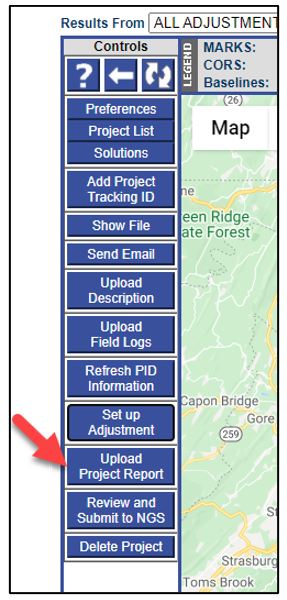
Fig. 12.29 Upload Project Report button on the Controls Bar on the Manager’s Page

12.7.6.2. Project Submission Checklist

To access and review the project submission checklist, click the button labeled “Review and Submit to IDB” on the Managers Page, as shown in Fig. 12.30.

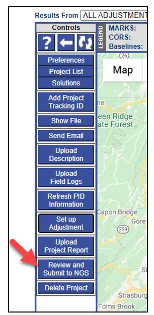
Fig. 12.30 The Review and Submit to NGS button on the Controls Bar on the Manager’s Page

When the Review and Submit to NGS button is clicked, OP runs a series of checks, including CHKOBS and OBSCHK (see 12.7.5 and 12.7.6). In the unlikely event errors are reported by the checking programs please contact the NGS Bluebook team for instructions before hitting the final submit button. If the user has any questions about how to resolve an error, or what is implied by an error message, feel free to contact the NGS Bluebook team as well.

OP also produces a checklist at this stage, showing any missing files. A successful submission will include the following items:

1. An NGS Project Tracking ID has been assigned to the project

2. All five (5) required Description files:

1. *.des

2. *.dsc

3. *.nbr

4. *.dis

5. *.err

3. Mark photos

4. Field logs, logically organized (preferred: digital field logs zipped into one file, hard copies scanned into one pdf )

5. Project report (pdf format required)

6. All five network adjustments run, checked, and verified for tolerance to project specifications

Make sure all required files have been successfully loaded into the project prior to submitting the project to NGS (example of missing files shown in Fig. 12.31). If any items are missing, OP will indicate any missing items.

Once all the checks are completed and files verified, the project can be submitted to NGS by clicking on the “Submit” button. Thank you for using OP to submit your GNSS project to NGS!

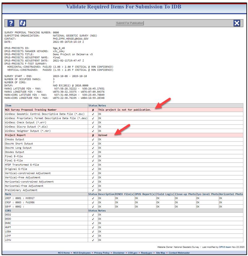
Fig. 12.31 Example of the result of a project check where two items are missing or incomplete

---

Footnotes:

4

Although not a formal constraint, this selection allows the user to determine an orthometric height by subtracting the Geoid Height from the Ellipsoid Height. Note that this will have important implications for vertical sigmas, and may lead to unintended adjustment statistics.

---